LESSON: The Normal Distribution
| Site: | Mountain Heights Academy OER |
| Course: | Introductory Statistics Q2 |
| Book: | LESSON: The Normal Distribution |
| Printed by: | Guest user |
| Date: | Friday, 6 June 2025, 12:37 AM |
Introduction
Most high schools have a set amount of time in-between classes during which students must get to their next class. If you were to stand at the door of your statistics class and watch the students coming in, think about how the students would enter. Usually, one or two students enter early, then more students come in, then a large group of students enter, and finally, the number of students entering decreases again, with one or two students barely making it on time, or perhaps even coming in late!
Now consider this. Have you ever popped popcorn in a microwave? Think about what happens in terms of the rate at which the kernels pop. For the first few minutes, nothing happens, and then, after a while, a few kernels start popping. This rate increases to the point at which you hear most of the kernels popping, and then it gradually decreases again until just a kernel or two pops.
Here's something else to think about. Try measuring the height, shoe size, or the width of the hands of the students in your class. In most situations, you will probably find that there are a couple of students with very low measurements and a couple with very high measurements, with the majority of students centered on a particular value.
All of these examples show a typical pattern that seems to be a part of many real-life phenomena. In statistics, because this pattern is so pervasive, it seems to fit to call it normal, or more formally, the normal distribution. The normal distribution is an extremely important concept, because it occurs so often in the data we collect from the natural world, as well as in many of the more theoretical ideas that are the foundation of statistics.

Characteristics of Normal Distribution
Shape
When graphing the data from each of the examples in the introduction, the distributions from each of these situations would be mound-shaped and mostly symmetric. A normal distribution is a perfectly symmetric, mound-shaped distribution. It is commonly referred to the as a normal curve, or bell curve.
Because so many real data sets closely approximate a normal distribution, we can use the idealized normal curve to learn a great deal about such data. With a practical data collection, the distribution will never be exactly symmetric, so just like situations involving probability, a true normal distribution only results from an infinite collection of data. Also, it is important to note that the normal distribution describes a continuous random variable.
Center
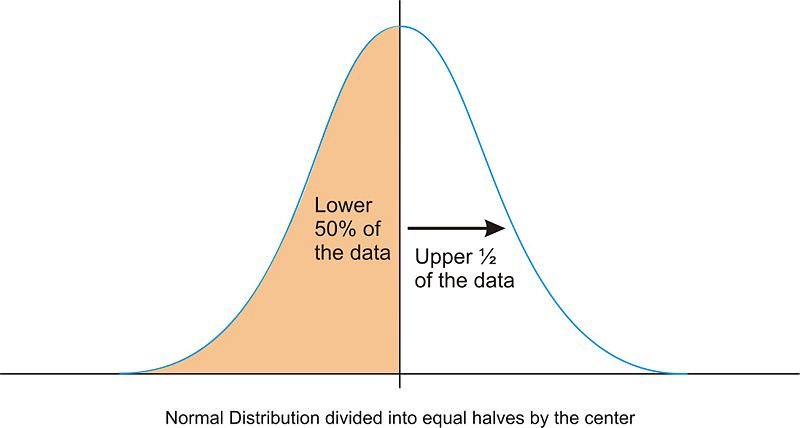
Due to the exact symmetry of a normal curve, the center of a normal distribution, or a data set that approximates a normal distribution, is located at the highest point of the distribution, and all the statistical measures of center we have already studied (the mean, median, and mode) are equal.
It is also important to realize that this center peak divides the data into two equal parts.

Spread
Let’s go back to our popcorn example. The bag advertises a certain time, beyond which you risk burning the popcorn. From experience, the manufacturers know when most of the popcorn will stop popping, but there is still a chance that there are those rare kernels that will require more (or less) time to pop than the time advertised by the manufacturer. The directions usually tell you to stop when the time between popping is a few seconds, but aren’t you tempted to keep going so you don’t end up with a bag full of un-popped kernels? Because this is a real, and not theoretical, situation, there will be a time when the popcorn will stop popping and start burning, but there is always a chance, no matter how small, that one more kernel will pop if you keep the microwave going. In an idealized normal distribution of a continuous random variable, the distribution continues infinitely in both directions.
Because of this infinite spread, the range would not be a useful statistical measure of spread. The most common way to measure the spread of a normal distribution is with the standard deviation, or the typical distance away from the mean. Because of the symmetry of a normal distribution, the standard deviation indicates how far away from the maximum peak the data will be. Here are two normal distributions with the same center (mean):
The first distribution pictured above has a smaller standard deviation, and so more of the data are heavily concentrated around the mean than in the second distribution. Also, in the first distribution, there are fewer data values at the extremes than in the second distribution. Because the second distribution has a larger standard deviation, the data are spread farther from the mean value, with more of the data appearing in the tails.

The Normal Distribution
We're focusing our learning on data sets that have a normal distribution (rather than skewed or random distributions). There is a lot of information that we can extract from data sets that are normally distributed. This is your introduction to the normal distribution and what we can learn from it.
Identifying Normally Distributed Data
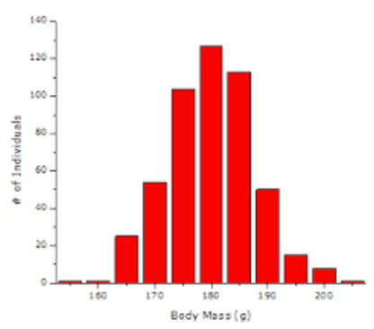
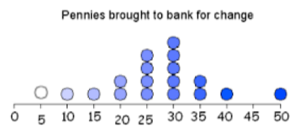
In order to determine if a data set is normally distributed it is best to graph the data on a histogram or a dot plot. If the shape of the data in the graph resembles the "bell" shape curve of a normal distribution, then it is safe to say the data is normally distributed.
Another way to check if data is normally distributed is to find the mean, median and mode of the data. If the mean, median and mode are all approximately equal, then the data is symmetrical; that means that data is normally distributed.
We can see that the two graphs shown below have normal distributions because they both have a "bell" shape and their measures of center are approximately equal.

Mean = 180.1 $$\approx$$ Median = 180 $$\approx$$ Mode = 180

Mean = 27 $$\approx$$ Median = 27.5 $$\approx$$ Mode = 30


