LESSON: Understanding Confidence Intervals
| Site: | Mountain Heights Academy OER |
| Course: | Introductory Statistics Q2 |
| Book: | LESSON: Understanding Confidence Intervals |
| Printed by: | Guest user |
| Date: | Friday, 25 July 2025, 6:19 PM |
Basic Overview of Confidence Intervals
In this lesson book we'll be learning about confidence intervals. Before we really dive into the topic though, watch this video so you have a basic idea of what confidence intervals are for, what they calculate and why they are important.
It might be helpful to watch this video more than once so you can really understand what she is explaining.
Here are the main points to understand:
1. We calculate the mean of a large population by taking a sample from that population first. If we select our sample randomly and give every member of the population an equal probability of being selected, then we can say that the mean of the sample is a good estimate of the mean of the population. However, if we select different sample groups from the same population, we will ALWAYS get different sample means. This is called sampling error.
2. When reporting the measures of a population (like mean, median, and range) it's good practice to give a range of possible values, instead of an exact value. For example, saying, "The estimated mean of the population is 140 grams." makes it sound like we are exactly sure of that number. But that's impossible due to sampling error. Rather, it's better to say, "The estimated mean of the population is between 137-143 grams."
3. A confidence interval communicates how accurate our estimates are likely to be.
4. The width of a confidence interval (or how accurate or estimate is) is determined by the following two things:
a) Variation: Are the members of the population similar? Or do they vary largely? Small variation means our confidence interval is larger. We are more sure our estimate is accurate.
b) Sample Size: If our sample size is large, then sampling error is reduced and we can have a larger confidence interval.
Introduction to Confidence Intervals

Confidence Intervals
The general concept of confidence intervals is pretty intuitive: It is easier to predict that an unknown value will lie somewhere within a wide range, than to predict it will occur within a narrow range. In other words, if you are making an educated guess about an unknown number, you are more likely to be correct if you predict it will occur within a wider range. This idea is reflected in the concept question above, where the reward is greater if you guess within a smaller range, because the contest creator knows that your chance of guessing correctly is much less if you have to guess within a smaller range.
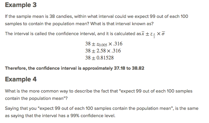
A confidence interval, centered on the mean of your sample, is the range of values that is expected to capture the population mean with a given level of confidence. A wider confidence interval is a greater range of values, resulting in a greater confidence level that the range will include the population mean. By convention, you will mostly be concerned with identifying the intervals associated with 90%, 95%, and 99% confidence levels.
Calculate the confidence interval by combining the sample mean with the margin of error, found by multiplying the standard error of the mean by the z-score of the percent confidence level:

It is common, but incorrect, to assume that a confidence level indicates the probability that the mean of the population will occur within a given range of the mean of your sample. A 95% confidence interval means that if you took 100 samples, all of the same size, and formed 100 confidence intervals, 95 of these intervals would capture the population mean.
The confidence level indicates the number of times out of 100 that the mean of the population will be within the given interval of the sample mean.
Calculating a Confidence Interval
Confidence Level & Confidence Coefficient
In this lesson video, I will explain the terms "confidence level" and "confidence coefficient" which were used in the last video to calculate the confidence interval.
Comparing Sample Means to Population Means
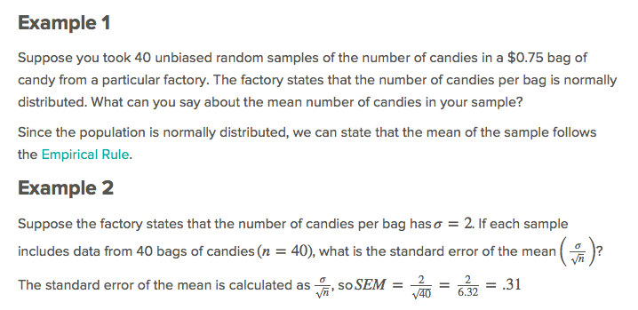
Suppose you took 100 unbiased random samples of the heights of U.S. women (recall that height is normally distributed), each sample containing 30 women. What can you say about the means of the samples $$(\bar{x}_{1},\bar{x}_{2},...\bar{x}_{100})$$ compared to the population mean?
Since height is normally distributed, we know that approximately 95% of women will have a height within two standard deviations of the mean (remember the Empirical Rule?). That means that out of 100 samples, we can assume that 95 of them will have a mean within 2 standard deviations of the population mean.
Predicting Population Means
Suppose the mean of the means of our 100 samples from this example is 5′5″, in other words, $$\bar{x}$$
Remember that since height is normally distributed, 95% of the values lie within 2 standard deviations of the mean, we need to identify that range of values.
- First we need to use $$Z_{\frac{a}{2}}\times \frac{\sigma }{\sqrt{n}}$$ to identify the margin of error (since we are looking for a 95% confidence level, this is the range of values within 2 standard deviations of the sample mean). Since $$\sigma$$
=1.5′′ , in this case we get $$1.96 \times \frac{1.5}{\sqrt{100}} = 1.96 \times \frac{1.5}{10}=1.96\times0.15\approx 0.3"$$ above and below $$\bar{x}$$.
- The interval then is 5′ 4.7″ to 5′ 5.3″, or .3 inches above and below the mean of 5′5″.
We can say that there is a 95% probability that the mean of our 100 samples would be within 0.3 inches either way of the population mean. Since the mean of our sample is 5′5″, we can say that the population mean is between 5′4.7″ and 5′5.3″ with 95% confidence.
Mathematically:
Plotting the Means of Samples
Suppose you plot the mean of each of your height samples on a graph, and drawing a line each way of the mean of each sample to represent 2 standard deviations. If you were to do this for 50 of the samples, you might end up with an image like the one below.
The image is a screen capture from the interactive applet at Bedford, Freeman, and Worth Publishing Group's website
At the top of the image is a normal curve. Each of the lines below the curve has a length that represents a 95% confidence interval, centered on the mean (in red) of the sample.
a. What is indicated by the lines that are all red in color?
The lines that are colored entirely red have a mean that is greater than 2 standard deviations away from the population mean. In other words, the mean of those two samples was not within the stated confidence interval (95%).
b. What value is indicated by the vertical red center line on each interval?
The vertical red center line represents the mean of each sample.
c. What does the "percent hit" number mean? How would it change if you were to continue taking more and more samples of 60 each?
The “percent hit” number indicates the percentage of times that the population mean was included in the confidence interval of sample means. If you were to continue plotting sample means and confidence intervals, the percent hit would approach 95%. In fact, here is the same graph after 1000 sample runs:
Earlier Problem Revisited
Suppose you were at a county fair and saw a large jar full of gumballs, maybe 1000 of them, with a sign that said “Guess the Number, Win a Prize!” If the rules of the game are that you could win a $10 prize by guessing within 200 gumballs either way, or a $50 prize by guessing within five gumballs either way, but you have to specify which prize you are trying for before submitting your guess, which would you choose?
This problem/question is meant to give you an intuitive feeling for the concept of a confidence interval or confidence level. It should be clear that you would have a greater level of confidencein trying for a $10 prize that you would win simply by guessing within +/- 20% of the number, than in trying for $50 by guessing within +/- 0.5% of the number!

Examples


Attribution
All texts in this lesson book were compiled from:


